When I want to do work with tensors, I use JAX in Python. But when I want to understand and visualize them, I use Wolfram Language. This article is an extended demonstration of why that is. :)
For a while now, I’ve spent a little time each week working through Pattern Recognition and Machine Learning (PRML), a textbook that teaches the fundamentals of ML. Wolfram Language has rich library functions for most of the concepts in the book, like matrices, probability distributions, and function minimization. And it plots!
But symbolic manipulation is the best part. I can write an expression and it stays an expression! When I calculate a derivative, I get to see the expression for the derivative.
Getting to this point wasn’t all sunshine and rainbows, though. My goal here is to succinctly summarize the lessons I’ve learned in how to use Wolfram Language to bridge the gap between the tensor work I already knew how to do in JAX/numpy, and the symbolic math I can do in Wolfram Language.
I’m going to assume that you have a similar background to mine: you know some linear algebra and have implemented neural networks in a framework like TensorFlow or JAX, but you’re not sure how best to represent those concepts in Wolfram Language for inspectability.
In a math text, I can define a tensor A and write ![]() to refer to its entries.
to refer to its entries.
However, in Wolfram Language, if I were to define a tensor a containing ![]() ,
, ![]() , and so on, the definition would be recursive and not evaluate very well:
, and so on, the definition would be recursive and not evaluate very well:
![]()
So my naming convention is to append “t” (for “tensor”) to the name that refers to the entire tensor. For example, I could define a tensor of shape {2,5} like this:
I leave a undefined so that expressions like ![]() remain unevaluated.
remain unevaluated.
Instead of writing out all the terms like that, though, I’d actually use Array, so that I can get the same result just by specifying the shape:
![]()
Neural networks are a nice first example because they’re genuinely useful, but not too complicated.
We can use the built-in NetGraph library to quickly create a visual representation of the network we want to build:
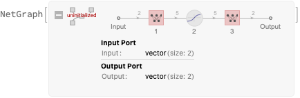
It takes 2-D inputs, has one 5-unit hidden layer with Tanh activation, and a 2-D output layer with linear activation.
While NetGraph is a great library, our goal is to understand all the math, and it’s tedious to disassemble a NetGraph as completely as we can if we define the network ourselves, like this:
The expressions for calculating output of the network are easy to write:
As is squared error loss:
I suppressed the printing of the expressions for the network outputs and loss above because, by default, Wolfram Language fully expands them until every defined identifier has been replaced by its definition. That’s handy sometimes, but not typically elucidating for expressions this large:
But MatrixForm and HoldForm can help. MatrixForm displays a matrix like a matrix, and HoldForm prevents identifiers from being expanded during evaluation.
They’re great for showing matrices as matrices:
And with a helper…
… we can render the network output expression in a way that communicates shape as well:
And the loss, of course:
![]()
Since everything’s defined symbolically, we can substitute values in arbitrarily.
There are dozens of variables across inputt, w1t, b1t, etc, so a function to assign them random values is helpful:
It works by returning a list of replacement Rules:
![]()
To actually substitute them in, we can use ReplaceAll. If we substitute in values for the inputs and all the network weights, we simply get the network’s output:
![]()
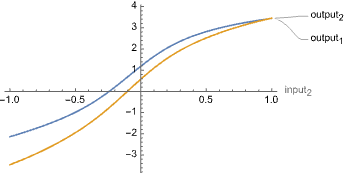
But we can get the output in terms of arbitrary subsets of the variables! We could plot the network’s response to changing just the second input:

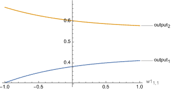
Or the network’s response to editing a single value in the hidden layer’s weight matrix:
![]()
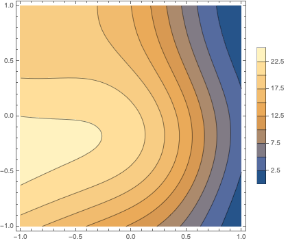
Since the input is rank-2 and loss is rank-1 (what a coincidence!), we can plot the loss over the input domain, assuming a target value of {0, 0}:
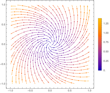
Or, since the input and output domains are both ![]() , we can view it as a transform and plot the vector field:
, we can view it as a transform and plot the vector field:
The usefulness of the above plots all depends on what you’re trying to learn when you decide to render them. The point is the flexibility and relative ease with which you can!
Of more conventionally practical importance, we can calculate the partial derivative of the loss respect to any of the variables, which we will most likely want if we ever decide to train this network…!
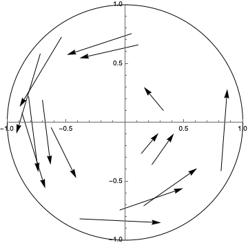
We need a dataset, so to start, I’m going to define one where the inputs are 2-D coordinates, and the outputs are those same coordinates rotated 45º counter-clockwise around the origin.
First, a function for performing the rotation:
And a function that generates an example for the dataset by picking a random point in the unit circle and rotating it:
We can use that to generate a whole dataset:
We can visualize it by mapping every example to an Arrow:
One way to find good network weights for our network using this dataset is with one of Wolfram Language’s built-in optimizers. For small datasets, NMinimize is enough to demonstrate that our little neural network can actually learn something.
Our goal is to minimize the total error of all examples in the dataset. That translates almost directly into code:

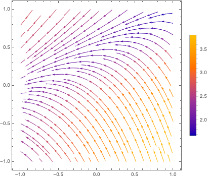
We can plot the transformation that the network learned, which if we eyeball the tangents in a stream plot, looks like the intended rotation:
If we plot the loss, we see that error is small everywhere in the unit circle that we trained on:
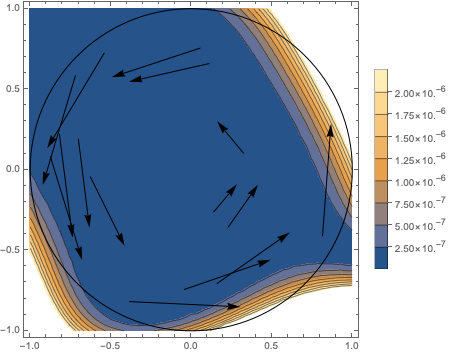
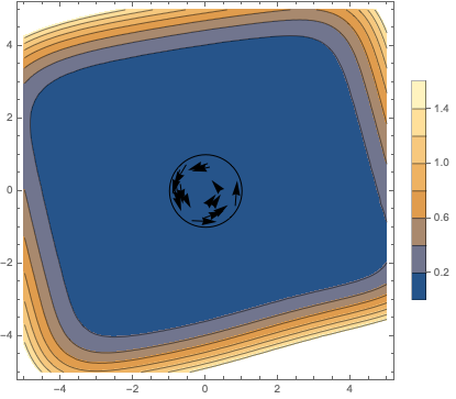
Unfortunately, you don’t have to zoom out very far to see that it doesn’t generalize, though you have to check the legend for the scale of the legend to notice:
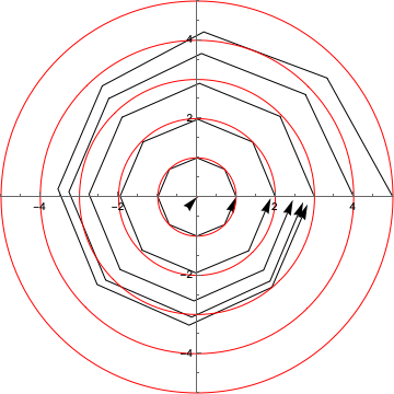
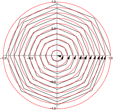
We can see the errors compounding more clearly if we feed the output of the network back into itself to generate trails, and overlay the circles that the trails would ideally trace:
Anyway, we did it!
Nah, this not a great way to do it if you care about training a realistic neural network. Like I said at the start, if I were trying to do real work, I’d be using a different tool—or at least, I’d be using completely different language constructs, like NetTrain.
Why isn’t it a good way, though? Because the function we’re asking the library to minimize is big. It contains a copy of the entire loss function (which contains the entire inference function) for every point in the dataset. It looks like this just for 3 data points:
I get tired of waiting for it even after only ~200 data points.
Meanwhile, NetTrain manages 10,000+ unique examples per second on my laptop:
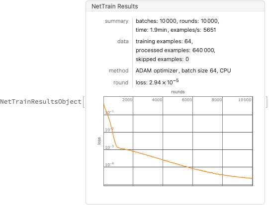
The final weights actually aren’t as good, though, even on the unit circle, though that’s a story for another day…
I’m publishing new sections as I go, so subscribe to know when there’s more!