Contrastive learning is the process of learning an embedding in which 1) items in the same class are close together and 2) items in different classes are far apart.
This notebook implements one of the simplest algorithms for doing so using the MNIST dataset of handwritten digits.
Dimensionality of the embedding space (min 2):
When debugging, it’s useful to only use some of the digit classes, so this lets you set the number of digit classes to include (min 1, max 10):
The algorithm below does no hard negative mining, so a large batch size is necessary to ensure that as many hard negatives are randomly included as possible:
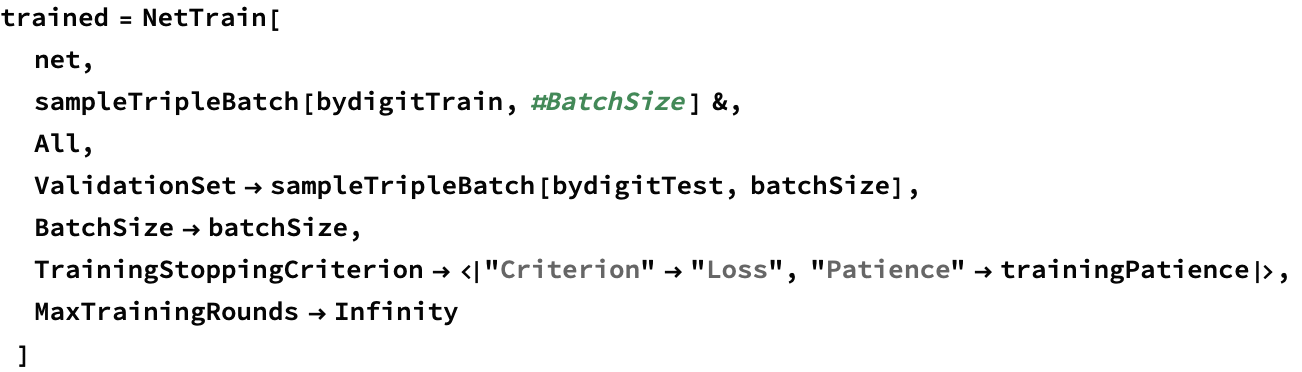
Training only stops when validation loss fails to improve for this number of batches:
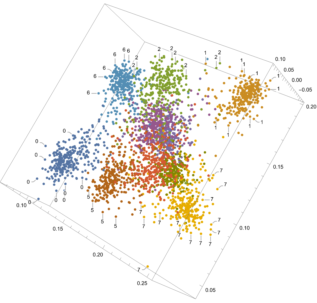
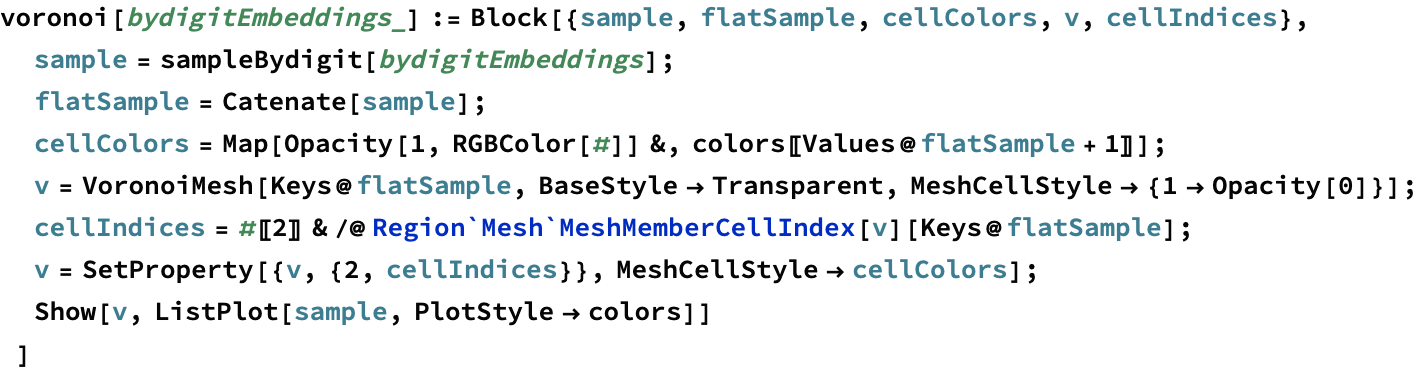
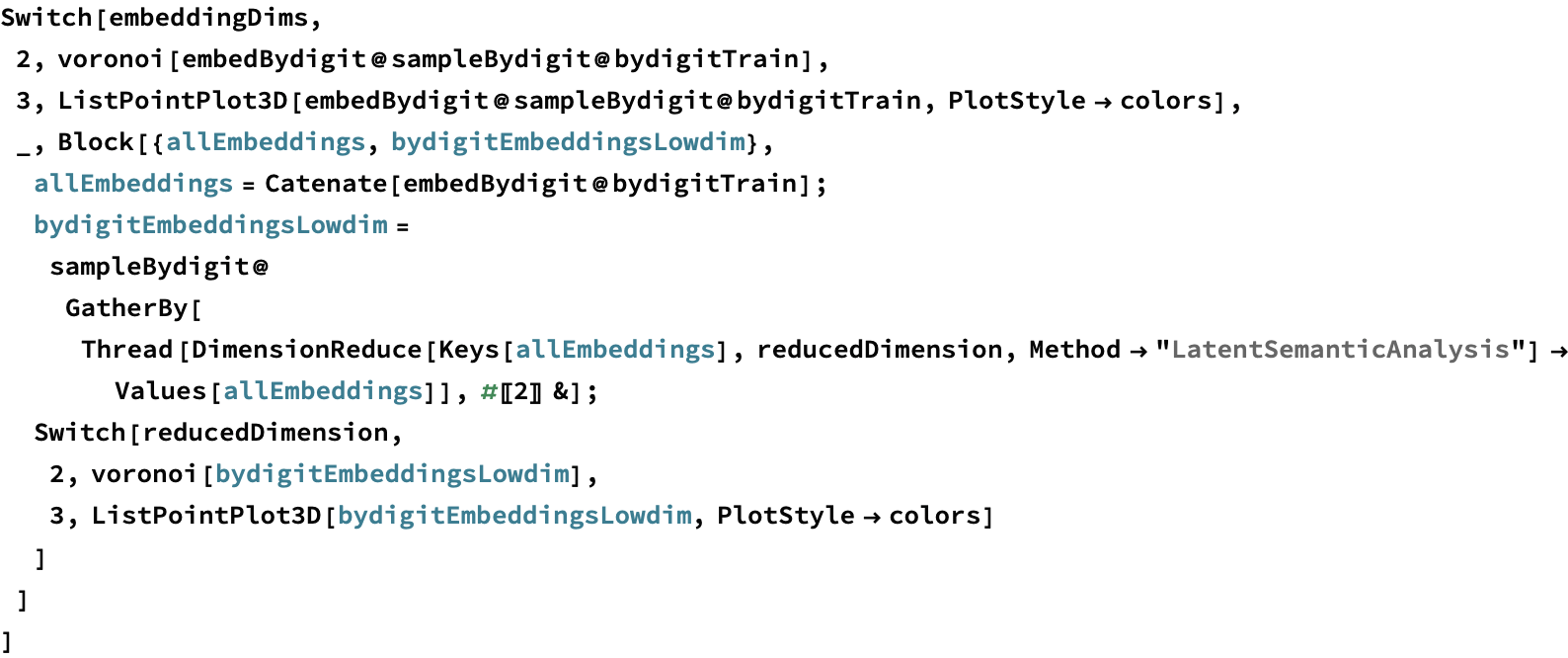
The number of dimensions to use in the visualizations of the resulting embedding space if embeddingDims is greater than 3. Setting this to 2 visualizes using a colored voronoi diagram. Setting it to 3 renders a 3-D point cloud.
How many examples to pull from each class in order to generate the visualization. Mathematica starts falling over if this goes above a few thousand.
![]()
Group the graining examples by digit, producing lists like {{{img → 0}, {img → 0}, …}, {{img → 1}, {img → 1}, …}}. This representation is useful throughout the notebook.
A triplet contains a random example (anchor), another example from the same class (positive), and a random example from a different class (negative).
![]()
![]()
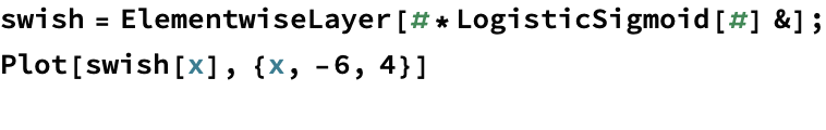
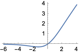
Swish is like Ramp with some extra curvature for that extra oomph.
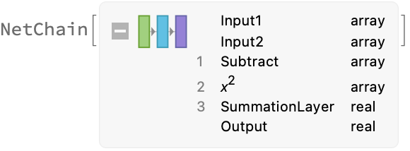
squaredDistanceLayer accepts two vectors and outputs their squared Euclidean distance.
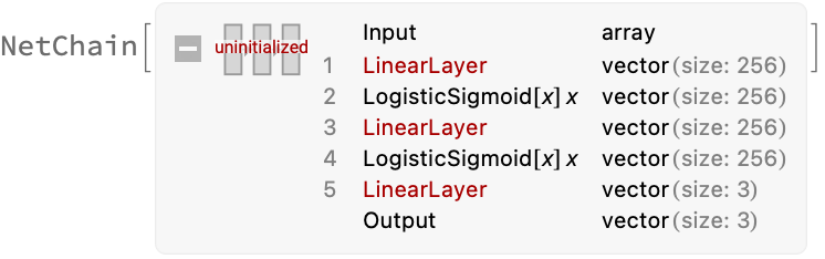
Define a projection from the input image to the embedding space. This could be fancier, but for MNIST, it doesn’t matter.
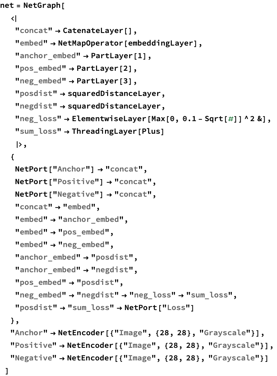
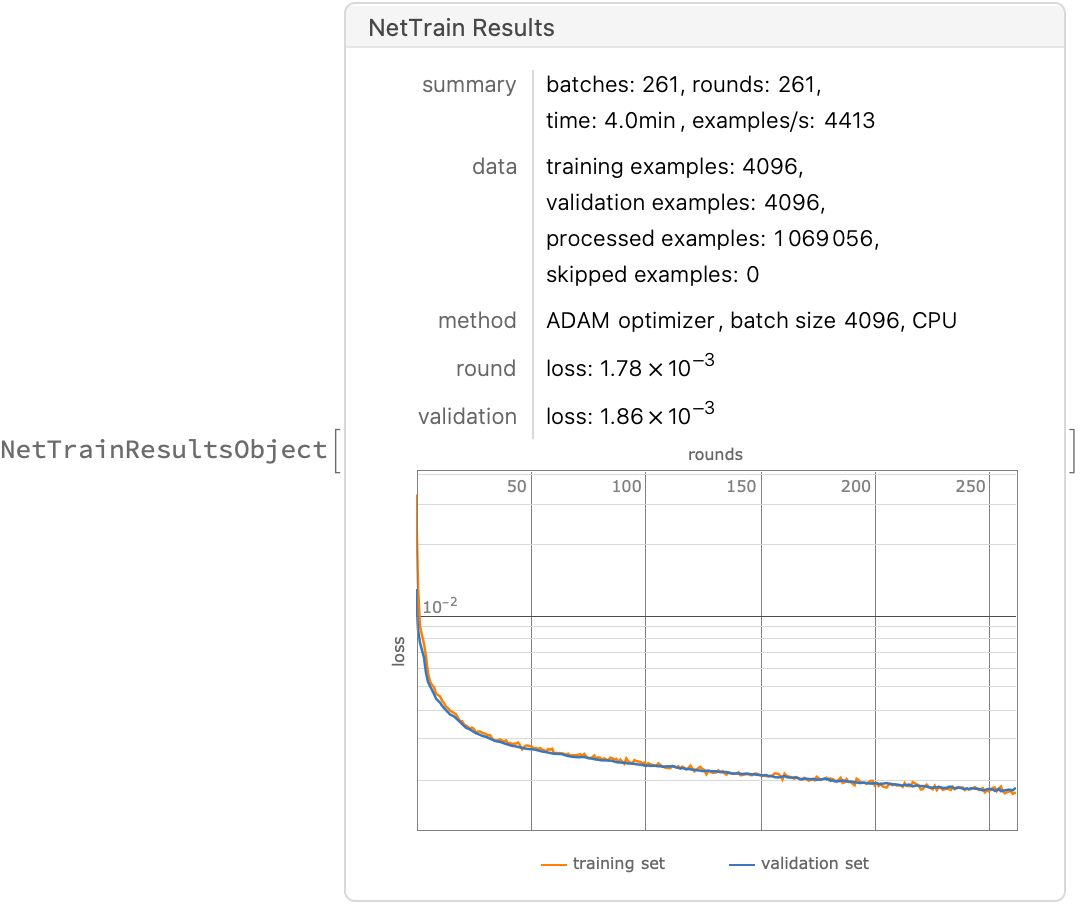
The network’s only output is the loss. Its purpose is to find weights for the embedding subnetwork that minimize the loss. We’ll extract the embedding subnetwork in the next section.
The closer the anchor and positive example embeddings are, the lower the loss. The further the anchor and negative example embeddings are, the lower the loss (up to a certain distance, after which it’s 0).
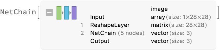
If we referred to embeddingLayer in the network three separate times, then each instance would get its own independent weights. To get just one embedding subnetwork, we must use NetMapOperator to create only one instance of embeddingLayer. The three images are concatenated, independently fed to embeddingLayer, and their embeddings are concatenated to form the output, which is deconstructed using PartLayers. (What would we do if we needed to use the output of one embedding as the input for a second embedding operation? I don’t know.)
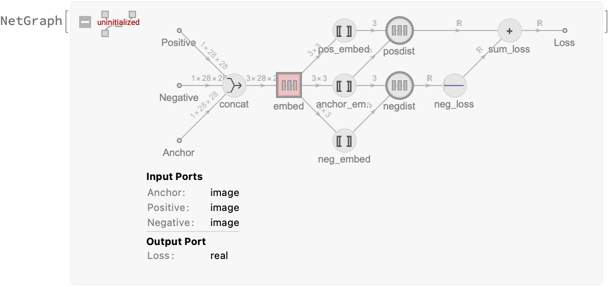
Extract the trained embedding sub-network by pulling it from the NetMapOperator named “embed”. There must be a nicer way to grab it, but I don’t know what it is.
A color map that I found slightly more legible than the built-in default:
This function visualizes an embedding in 2-D by rendering a Voronoi diagram of the examples in embedding space and giving each class a separate color.
Visualize the embedding space according to the config at the top. 2-D is voronoi, 3-D is point cloud. When the embedding space has more than 3 dimensions, SVD is used to reduce its dimensionality to reducedDimension first.